How big will an influenza outbreak be?
Motivation
Before we start modelling the severity of influenza seasons, we investigated the state-of-the-art for this field. As the leading national public health institute in the United States and one of the world’s premier infectious disease surveillance bodies, the Centre for Disease Control (CDC) represents the status quo in influenza modelling. The CDC currently deploy an adaptation of Serfling’s method 1, which uses cyclic regression to model the weekly proportion of deaths from pneumonia and influenza. Adaptations to the basic model have incorporated indicators such as counts of patient visits for influenza like illness (ILI) 2 3. However, regardless of modern modifications, the methodology is limited by its unfounded assumption that observations are independent and identically distributed.
In this contribution, we attempt to shift the methodology towards the Bayesian framework in order to provide better epidemic thresholds that are adjusted for seasonal effects. In doing so, we build prior and observation models for the number of individuals infected by influenza within a specific region. After building the models, we simulate from the prior to test the model’s performance and ensure the prior model is sufficiently grounded in reality to produce justified posterior inference. Once we are satisfied with the model we deploy Approximate Bayesian Computation (ABC) to generate approximate posterior samples and proceed to make probabilistic statements to inform policy makers.
Prior Elicitation
We begin by outlining the prior and observation models in this setting. Whilst the systematic use of parametrised distributions is not always justifiable, when building the prior we arbitrarily restrict ourselves to a parametrised density where we can make subjective evaluations of the parameters in line with our knowledge of the world.
Prior Model
We build a model for the number of individuals infected by influenza in a given week for a two year period. Whilst the model is agnostic to geographical location, we focus on specifying the prior distribution in line with European influenza cycles. The parameters are \(\Theta = (X_{1:104},\mu, \theta, \alpha, \rho, \ell)\). The notation is defined as follows: \((X_{1:104}) := (X_1,\ldots,X_{104})\), where \(X_i\) is the number of positive influenza samples recorded in week \(i\), and the others are parameters for the model, as defined below. Using these parameters, we model the weekly flu process \((X_i)_{i=1}^{104}\) over a 2 year period (for example 2018 to 2019) as a weekly mean with an autoregressive (AR) process. By considering the seasonality of infection count we use a single AR process for each winter, since each winter has a number of hidden variables. For example, the strands of influenza active, health care spending, temperature and so on differ depending on the year. By only considering short time periods, we lower the risk of being affected by the change of these hidden variables.
Putting this all together, we have \(X_t|X_{t-1},\phi = m_t+y_t\) with \(y_t \stackrel{}{\sim} AR(\rho,50)\) and \(\phi = (\mu, \theta, \rho, \ell, \alpha)\). The mean in week \(t\) is given by
That is to say, the weekly mean is a baseline infection count \(\mu\), with \(\theta t\) to describe the secular trend, and a suitably scaled and lagged sine function to capture seasonality.
The prior \(\pi(\Theta)\) is composed of the following:
for \(t \in \{2,...,26,28,...,78,80,...,104\}\).
Given this prior model we have the following decomposition:
Observation Model
We model a two year period above and make predictions for the second year given the observations in the first. The data from the first year involves some noise due to poor data collection and miss-classification of illnesses, that is to say that the observed data \(Y_i\) has the form
where \(\epsilon_{i} \stackrel{iid}{\sim} \mathcal{N}(0,1)\). Thus we have
Simulating our prior model
As our prior model is a reductive representation of a complex random phenomena, it is vital to evaluate the model for likeness to the real world to ensure our posterior inference is justified.
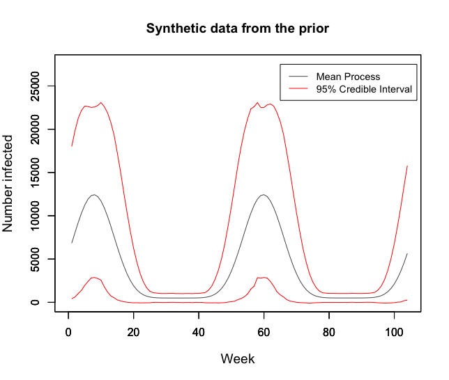
We first consider 100,000 samples from the prior model in the below figure. This graph demonstrates likeness to real observed data for Europe over the past 5 years. Additionally, the credible intervals plotted show a sufficiently large range of realisations. The mean weekly flu count is 3934 (Credible Interval: 1313, 6629) which provides a reasonable fit to the reality of the weekly average of 4611 patients in 2018 in Europe.
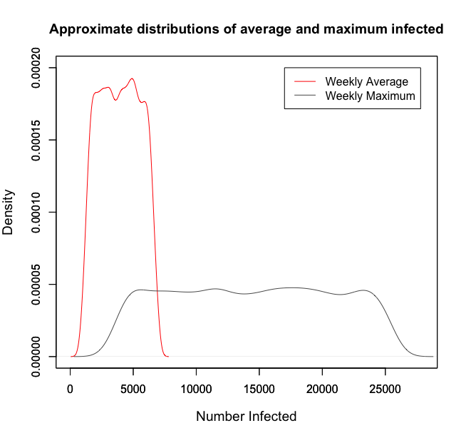
It is important to scrutinise the prior for informativeness with respect to the quantities we are particularly interested in. In the below figure, the approximate distribution of average and maximum counts for 100,000 samples are given. Both are satisfactory since they fall roughly uniform across wide intervals. The weekly average of 4611 in 2018 falls in the range of high density for the average, and the European 2018 maximum of 19,074 patients infected also sits in the high density region of the approximate maximum. Both distributions reflect reality well and do not over-inform.
A Quick Remark
When choosing a prior it is important to consider alternatives. In this project a range of distributions for each of the parameters \((\alpha, \rho, \ell, \mu, \theta)\) were considered in order to represent different states of knowledge. We verified that the results of our analysis were not sensitive to this range of priors. For example in our choice of \(\mu\), which provides the base-level for the weekly mean \(m_{t}\), we considered variants of uniform, normal and triangle distributions, including \(\mathcal{N}(10000,3),\mbox{Unif}(3000,25000)\) and \(\text{Tri}(3000,25000,10000)\). We observed reasonable similarity between the distributions and ultimately decided to work with the uniform distribution since it best represented our prior beliefs.
Model Choice
We are interested in understanding whether or not our current model, \(\mathcal{M}_{1}\), is adequate. In doing so, we compare its performance with alternative models whose difference with our current model is the sine function raised to a high power. That is, for alternative models \(\mathcal{M}_{2}, \mathcal{M}_{3}, \mathcal{M}_{4}, \mathcal{M}_{5}\) and \(\mathcal{M}_{6}\), we alter the weekly mean number of influenza positive virus as:
Note that all models considered are even powers of sine as we know the weekly mean number of influenza positive virus to be always positive. Here a finite number of model comparisons is made. If one wants to consider an infinite number of models a more delicate construction of the unconditional probabilities \((p_{i} : i \in \mathbb{N})\) is required (for example adhering to notions of coherence). Assuming an equal prior weighting, we progress to consider Bayes factors.
Bayes factors depend on estimates of the marginal likelihood for the observation in question, that is, the first year falling in line with recorded data. We make use of the following consistent estimator:
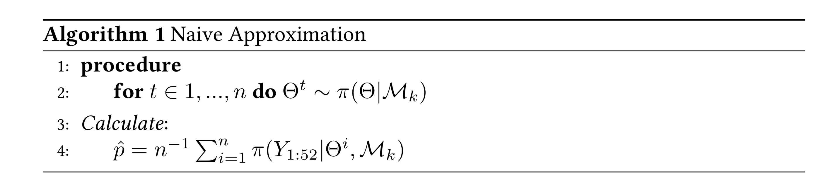
When implemented using \(n=100,000\) the approximation produced unstable results despite efforts to reduce computational underflow. To assess the evidence for accepting \(\mathcal{M}_{k}\), \(k\neq 1\), over \(\mathcal{M}_{1}\) we compute the Bayes factor for the best performing of \(\mathcal{M}_{2},...\mathcal{M}_{6}\) against \(\mathcal{M}_{1}\). In 10 runs we realised a range of \((0.004,12.656)\) with the Naive approximation. However, the particular \(\mathcal{M}_{k}\) with the best performance was consistently \(\mathcal{M}_{1}\), so we proceed with \(\mathcal{M}_{1}\).
Posterior sampling
Now that we are confident with the prior model, we proceed to generate approximate samples of the posterior distribution given observed European data. Whilst it would be possible to generate true posterior samples, for example by using Metropolis-Hastings and assessing the quality of fit with ACFs, trace plots, and checking that marginal distributions agree, we instead deploy ABC to generate approximate uncorrelated samples.
Approximate Bayesian Computation
With the aim to make probabilistic statements about 2019 we deploy
approximate Bayesian computation to target the posterior. In doing so,
we generate samples from \(\pi(\Theta|Y_{1:52})\) where
\(Y_{1:52}\) are given in influenza_activity.csv.
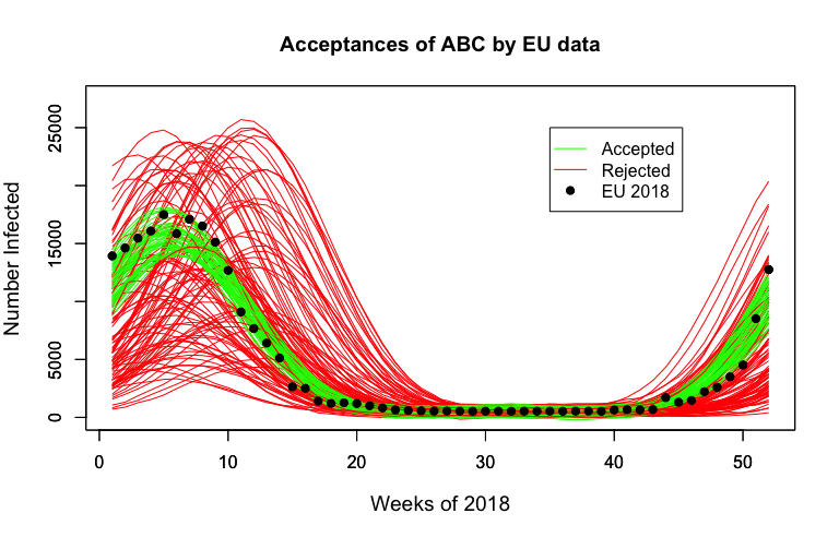
Below we observe the first year of some synthetic data, with samples accepted by ABC in green. These samples provide a satisfactory fit to the observed process.
Results
Using the posterior distribution we can inform policy makers about the probable magnitudes of the outbreaks, allowing for improved emergency planning and resource allocation. This methodology also provides an opportunity to look at the posterior for different regions of a country. Medical professionals can then strategically allocate their resources to regions with a higher probability of outbreak.
To demonstrate its usefulness, we consider 2018 model predictions given 2017 cycle observations. While we observe the peaks to be consistently above the mean prediction, we find that the observations for 2018 consistently fell within our tight Highest Posterior Density (HPD) interval. Given that the European Centre for Disease Prevention and Control recognised 2018 as a reasonably large season, we are encouraged by the fact the observations still fell within our bounds 4.
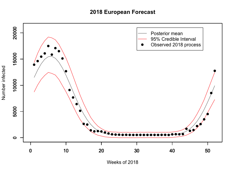
These results demonstrate our model’s usefulness; with a traditional model based off Serfling’s method, we could not have estimated the amount of extra resources required to manage large seasons such as this one, but our model gives a credible interval which can even account for these. We envision that policy makers could use our model to make sure that they are well prepared for large events whilst also ensuring that they do not overbudget.
Using 2018 observations for 2019 predictions, we observe an expected maximum number of viruses testing positive for influenza at 14,487 with a 95% credible interval of (3882,24675) in the prior. This expected maximum shifts to 19,413 in the posterior with a 95% credible interval at (14507,20085), putting the 2019 flu season on track to be about as large if not larger than the 2018 one. Below we also produce the expected flu cycle for 2019 with 95% HPD intervals.
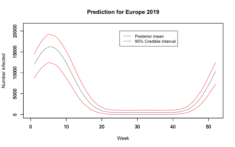
We also believe that this could provide an alternative epidemic threshold to that currently used by the Centre for Disease Control; if we were to find that the number of infections lies outside the HPD region, this would be an indication that we are failing to control the outbreaks and on the verge of an epidemic, and suitable measures should be taken.
Shortcomings
Whilst we achieved success in developing a model that reframed and extended the existing approach, there are a few shortcomings to be mentioned. Firstly, it is generally difficult to assess whether arbitrary features of the prior predominate our posterior analysis. The question of robustness has been tackled in the literature and we could extend our models by considering the prior belonging to a class of distributions as proposed by Berger’s classification 5. Attempts could then be made to derive bounds on posterior quantities and hence produce analysis that is less sensitive to the choice of prior.
Beyond criticism of the arbitrariness and importance of the prior, we must also consider the use of ABC. The applications of ABC are often based on improved versions of the basic rejection scheme 6, and have already yielded valuable insights into questions concerning the rate of spread of pathogens 7, 8, although we go beyond past applications that have typically focused on parameter estimation rather than posterior prediction. In our case, ABC provides the benefit of independent samples. However, true posterior samples could be found by the implementation of Hamiltonian Monte Carlo 9.
Finally, the Naive approximation of Bayes factors in this setting proved unstable. Future work could focus on deploying more stable estimators for the marginal likelihood, such as a Harmonic approximation.
- 1
Robert E. Serfling. (1963). Methods for Current Statistical Analysis of Excess Pneumonia-Influenza Deaths. Public Health Reports (1896-1970), 78(6), 494-506. doi:10.2307/4591848
- 2
L.Simenson, K. Fukuda, L. B. Schonberg, and N. J. Cox. The impact of influenza epidemics on hospitalizations. The Journal of Infectious Diseases, 181:831–837, 2000.
- 3
F.C. Tsui, M. M. Wagner, V. Dato, and C. C. H. Chang. Value ICD-9-Coded chief complaints for detection of epidemics. In Proceedings of the Annual AMIA Fall Symposium, 2001.
- 4
- 5
(Berger’s (1990a))
- 6
Beaumont, M.A. et al. (2002) Approximate Bayesian Computation in population genetics. Genetics 162, 2025–2035
- 7
Tanaka, M. et al. (2006) Estimating tuberculosis transmission parameters from genotype data using approximate Bayesian computation. Genetics 173, 1511–1520
- 8
Shriner, D. et al. (2006) Evolution of intrahost HIV-1 genetic diversity during chronic infection. Evolution 60, 1165–1176
- 9